In addition to the industry standard PD0 data format, Origin ADCPs also log high-fidelity proprietary data formats, A-gram and B-gram. In this blog, we introduce and explain the core content of the B-gram data format produced by Origin ADCPs.
Most of the time, we focus on the water velocity measurements that an ADCP makes and the application of those measurements. However, that’s just the result of a set of steps in a complex process of data acquisition and processing that an ADCP performs under the hood.
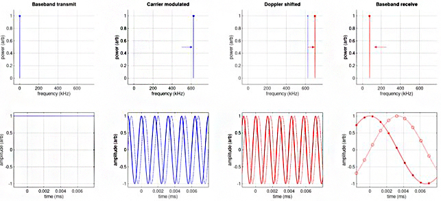
Let’s remind ourselves of how an ADCP works. The ADCP transmits an acoustic signal from its transducers and this signal has a certain frequency – see the first plot in Figure 1. The frequency is just the number of times the face of the transducer vibrates back and forth per second as it delivers sound into the water and is sometimes called the ‘carrier frequency’. A human ear can hear sound between about 20 Hz-20 kHz; Origin 65 and Origin 600 have carrier frequencies of 62.5 kHz and 625 kHz respectively.
The transmitted signal can be scattered by particles in the water. Some of this scattered signal makes it back to the same transducer that did the original transmission – this process is called ‘backscatter’. If the signal is backscattered by particles that are moving, the frequency of the original signal is altered. See the second and third plots in Figure 1.
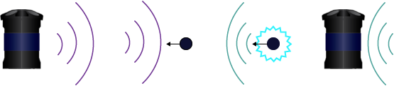
On reception by the transducer, this causes the transducer to vibrate at the frequency of the backscattered signal, and the vibration results in a transducer voltage that changes at that same frequency – see the last plot in Figure 1. The ADCP electronics can then measure and sample the voltage for processing; in essence, this sampled voltage is the main component of B-gram data.
A simple example
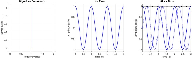
Let’s consider a simple case first. Suppose we have a signal that has a frequency of 1 Hz.
The left panel in Figure 2 below shows what that signal looks like in a plot of power versus frequency. You can see that there is power at 1 Hz (shown by the blue line and dot), but at no other frequencies – we call this a ‘tone’ because only one frequency is present in the signal.
The middle panel shows what this signal looks like in a plot of amplitude versus time. The blue line moves up and down once per second, so over the three seconds shown, the 1 Hz signal moves up and down three times. In this simple example the signal does not lose any strength, so how is it that the amplitude is zero at 0.25s, 0.75s, 1.25s, and so on. The sound surely can’t just appear and then disappear? In fact, it doesn’t – we just haven’t shown the full story yet.
Now look at the panel on the right. Even a simple signal like a tone has two parts to it – the first part in solid blue (the same as shown in the middle plot), and a second part that is offset from the first (dotted blue line). We call the first part I and the second part Q, which are formally called the ‘In phase’ and the ‘Quadrature’ components. You can see if we calculate the power in the signal (by squaring I and Q, summing them, and then taking the square root), the black line shows that the total power in the signal doesn’t change, which makes a lot more sense!
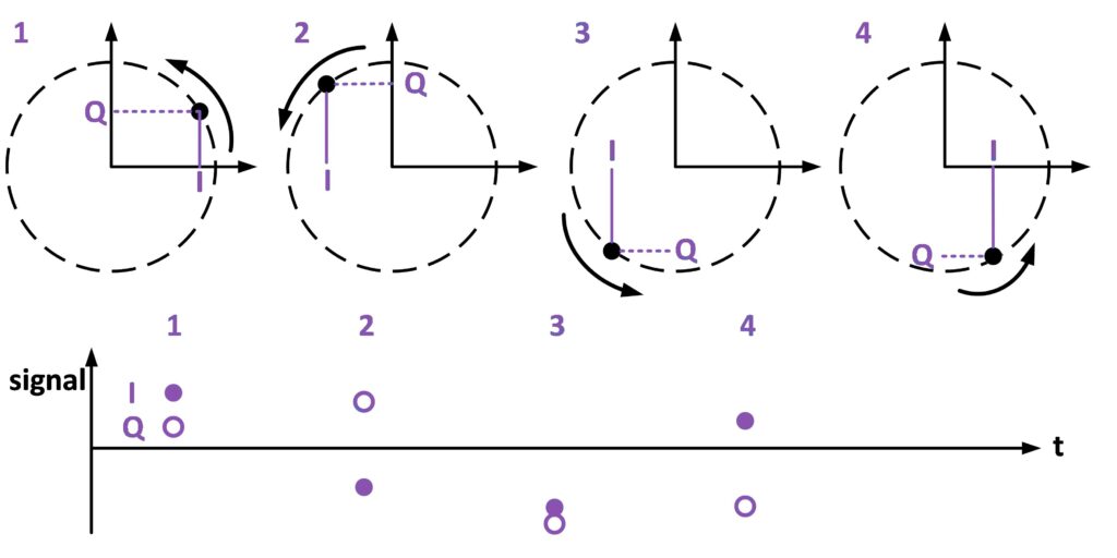
To understand what I and Q represent, see Figure 3. Think of the signal as a dot that travels round and round a circle as time increases – in Figure 3, we’ve shown four time steps, labelled 1 to 4. The radius of the circle is like the power in the signal, which in this simple example doesn’t change. I is the position of the dot along the x axis, and Q is the position of the dot along the y axis. So, if we only measure one of them, we can’t fully describe the circle and we can’t measure all of the signal.
We don’t have to measure I and Q continuously; that would take up a lot of disk space! The right plot also shows dots and circles which correspond to samples of I and Q – if we sample at least twice as fast as the carrier frequency, we have enough information to reconstruct the signal later for analysis (the technical term for this is the Nyquist criterion). It’s also important to note that each pair of I and Q samples are collected at the same instant – the dots and circles line up in time.
The main component of the B-gram data format produced by Origin ADCPs holds samples of I and Q; this is essentially raw acoustic data – it hasn’t even been processed into Doppler velocities yet. There is always one B-gram per ADCP beam, per ping. Metadata such as device serial number, details of measurement schedule, pressure and temperature measurements by internal sensors are also included in the B-gram format – see the Integration Manual IM-8375 for a full description of the data format.
Doppler shifting
So far, we have described what I and Q are referring to a simple tone signal. However, ADCP is all about measuring water velocities, which come from the frequency shift that occurs when the transmitted signal is scattered by a moving particle in the water column. This frequency shift is called the Doppler effect and is commonly observed in the change of pitch when an emergency vehicle siren is moving towards or away from you.
Let’s dig a bit deeper into how an ADCP works under the hood. Check out the top left panel of Figure 4 below. This plot shows the simplest possible signal, one that maintains horizontal alignment – you can see this in the plot below which shows the signal as a function of time (we’ll consider more realistic signals later). This is what the ADCP electronics might produce before transmitting via the transducers. Such a signal is normally produced at a frequency much lower than the carrier frequency and it is often called a baseband signal.
The transducers themselves are tuned to a particular carrier frequency, like 62.5 kHz and 625 kHz for Origin 65 and Origin 600 respectively. So, we can’t just transmit a baseband signal. What we must do first is modulate or up-mix the baseband signal to the carrier frequency. When this is performed in the ADCP electronics, you get the signal shown in the ‘Carrier modulated’ column of plots.
The top panel shows the input signal as a function of frequency, and in this case the signal has been modulated to 625 kHz – this just means that the baseband signal is shifted so that it is centred on the carrier frequency. The lower panel shows the modulated signal as a function of time. You can see that the signal is still a tone because only one frequency is present. And now that the tone has been modulated to the carrier frequency, the transducers can deliver it into the water. As before, the solid line corresponds to I and the dashed line to Q.
The next column of plots labelled ‘Doppler shifted’, shows what happens when the signal backscatters off a moving particle. In this example, the transmitted signal (blue) is Doppler shifted to a frequency 75 kHz higher than the carrier (red); this shift is much larger than what you see in reality! If you look carefully at the plot just below, the red lines move up and down a bit faster than the transmitted signal because of the Doppler shift that occurred when the signal was scattered by the moving particle.
When the backscattered signal reaches the ADCP, the transducer vibrates, inducing a voltage in the electronics. At 625 kHz you’d need fast electronics to sample that signal, so instead the signal is first demodulated or down-mixed. This just means that the received signal is shifted in frequency by an amount equal to the carrier frequency. If there were no Doppler shift in this example, this demodulated signal would be located at 0 kHz, and we’d see the same received signal as we saw in the leftmost pair of plots.
Instead, we see from the top right plot that the received signal has a frequency offset from zero by the exact amount due to the Doppler shift (75 kHz in this example). So, when we plot it as a function of time in the bottom right plot, the signal now moves up and down. We can use this information to calculate the Doppler shift, and hence how fast the scattering particle was moving. As in the first example, I and Q are shown as solid and dashed lines respectively, and the dots correspond to where the digital electronics sample this signal. Once again, these I and Q samples are what is logged in the B-gram data format.
The effect of bandwidth
The use of tones in ADCP data is often referred to as ‘narrowband’ ADCP measurements, but this isn’t the only type of signal that can be used. In our final example, we consider signals that (unlike tones) contain more than one frequency component. We call these ‘broadband’ signals.
Have a look at Figure 5. It is identical to Figure 4, except that the baseband signal now contains a range of frequency components shown by the shaded area; see the top left plot. If you look at the plot below, this now shows a signal that varies with time.
When this signal is modulated by the carrier frequency (second column of plots), as with the tone, the whole signal just shifts up so that its band of frequencies is centred on the carrier. In the lower plot, the signal now contains two components: the high frequency undulating at the carrier frequency, and an ‘envelope’ that has the same shape as the baseband signal (we’ve only plotted I here otherwise the plot would get a bit busy!).
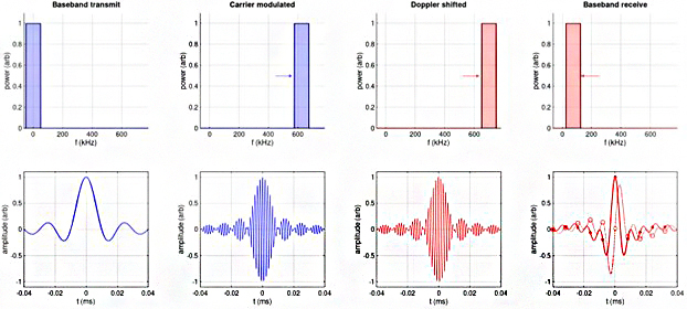
The next column of plots shows what happens when the signal is Doppler shifted by 75 kHz as before. The top plot shows that the frequency band shifts up by another 75 kHz due to the Doppler shift, while the lower plot shows (if you look hard!) that the baseband signal ‘envelope’ has not changed, but the high frequency component is now moving faster than the unscattered signal; again, we’ve only plotted I.
The final column of plots shows both I and Q once the backscattered signal incident on the transducer has been demodulated to baseband. We can see that the structure is different from the input signal, and like the tone example above we can use the shape of this signal (via the I and Q samples) to determine what the Doppler shift was, and hence the velocity of the scattering particle. In fact, this is exactly what the Origin ADCP processing does to convert the I and Q data held in B-grams into the Doppler velocities stored in our other proprietary format, A-gram.
To find out more about B-gram, or if you have any further queries surrounding our proprietary data formats, please get in touch.
Further information about the ADCP family of products can be found here. You can also request Origin 600 ADCP related manuals here.